About METEX

To calculate an air parcel trajectory, METEX uses meteorological data for derivation of displacement of the air parcel. The calculation mainly involves spatial and time interpolation to obtain values of meteorological variable at a specific position and time from available data, and involves time integration to estimate the motion of an air parcel. The procedures are outlined as follows:

  1. Specify the latitude, longitude, altitude, and time as initial conditions.
  2. Read meteorological data from files whose time intercept the initial time and find the grid box that enclose the given latitude, longitude, and altitude.
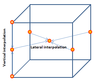
  3. Calculate values of meteorological variables for the same latitude, longitude, and altitude for those times of the two meteorological data files by spatial interpolation using data on the eight corners of the grid boxes.
  4. Calculate values of meteorological variables for the time and position of air parcel by time interpolation from the two spatially interpolated values.
  5. Estimate the integration time step based on wind velocity at the time and position obtained by step 4.
  6. Estimate the new position of the air parcel from wind variables by time integration using the specified calculation model.
  7. Repeat steps 2 to 6 for a specified period.

Meteorological Data

To calculate trajectories, METEX uses meteorological data provided by NCEP (National Centers for Environmental Prediction).

Data
1979 - 2010
NCEP Climate Forecast System Reanalysis (CFSR) 6-hourly Products, January 1979 to December 2010 (DOI: 10.5065/D69K487J)
2011 - present
NCEP Climate Forecast System Version 2 (CFSv2) 6-hourly Products (DOI: 10.5065/D61C1TXF)
Time Resolution 3 hours
Spatial Resolution 0.5 x 0.5 degree
Pressure Level 1000, 975, 950, 925, 900, 875, 850, 825, 800, 775, 750, 700, 650, 600, 550, 500, 450, 400, 350, 300, 250, 225, 200, 175, 150, 125, 100, 70, 50, 30, 20, 10, 7, 5, 3, 2, 1-hPa

Calculation Model

・3D-wind (kinematic) model

The kinematic model assumes that an air parcel's trajectory is dominated by u- and v-wind and the vertical pressure velocity.

In spatial interpolation, a variable is first interpolated along the vertical grids to the specified vertical position, which may be represented by geopotential height, pressure, or any hybrid coordinate; and then interpolated laterally to a specified latitude and longitude. The assumption for vertical interpolation is that variables vary linearly with height; and the assumption for laterally interpolation is that variables vary linearly with latitude and longitude.

Kinematic model

・Isentropic model

The isentropic model assumes that the vertical motion of an air parcel is confined on the isentropic surface with uniform potential temperature.

First of all, the initial altitude of an air parcel is converted to the potential temperature at its position by interpolation and by iteratively re-evaluating the potential temperature until the altitude estimated by interpolation on the isentropic surface equals the initial altitude within a given accuracy.

After the initial potential temperature is determined, the isentropic surface is treated as a flat plane in lateral interpolations for u- and v-wind. The flat-plane assumption is valid because the distance between vertical grids is generally much smaller than that between lateral grids.

Isentropic model

Time Integration

Metex uses the Petterssen method (1954, Weather Analysis and Forecasting. McGraw-Hill Book Company, New York. p221-223) to calculate a parcel's move from time \(t\) to \(t+\Delta t\).
When the position vector at time \(t\) is \(\boldsymbol{L}(t)\) and the velocity vector \(\boldsymbol{Γ}(L,t) \) at time \(t\) located at \(L\), the parcel's position vector \(\boldsymbol{L'}(t+\Delta t)\) at time \(t+\Delta t\) can first be estimated by the following equation.

$$ \boldsymbol{L'}(t+\Delta t) = \boldsymbol{L}(t) + \boldsymbol{Γ}(L,t) \times \Delta t $$

The parcel's position vector \(\boldsymbol{L}(t+\Delta t)\) at time \(t+\Delta t\) is obtained by

$$ \boldsymbol{L}(t+\Delta t) = \boldsymbol{L}(t) + 0.5 \times (\boldsymbol{Γ}(L,t)+\boldsymbol{Γ}(L',t+\Delta t)) \times \Delta t $$

where \(\boldsymbol{Γ}(L',t+\Delta t)\) is the velocity vector of the air parcel at time \(t+\Delta t\) located at \(L'\).

Integration Time Step

To achieve both good accuracy and fast computing, METEX adopted FLEXTRA's method of using flexible time steps in integration. The time step \( \Delta t \) is determined according to the horizontal wind velocity (\(u,v\)) by

$$ \Delta t = \frac{\Delta D}{CFL \times \sqrt{u^{2} + v^{2}}} $$

where \(\Delta D\) is the distance between two adjacent lateral grids and \(CFL\) stands for the Courant-Friedrichs-Lewy criterion. METEX uses the value 5 internally for \(CFL = 5\).

References

For more information on the methods and results of the trajectory calculations, please refer to the following paper.