Metadata
Title
Fish–prey interactions in, and associated data from, a temperate stream of the Yura River, Kyoto, Japan
Authors
Hikaru Nakagawa1 and Yasuhiro Takemon2
1Field Science Education and Research Center, Kyoto University,1 Onojya, Miyama, Nantan, Kyoto, 601-0703, Japan, hikarunakagwa@icloud.com (Corresponding Author)
2Disaster Prevention Research Institute, Kyoto University, Gokasyo, Uji, Kyoto, 611-0011, Japan, takemon.yasuhiro.5e@kyoto-u.ac.jp
Abstract
Although quantitative data on interspecific interactions within complex food webs are essential for evaluation of assumptions, hypotheses, and predictions of ecological theories; empirical studies yielding quantitative data on complex food webs are very limited. Ecological information on body size, habitat use, and seasonality of the component species of food webs aids in determining the mechanisms of food web structures. Ideally, ecological information on component species should be obtained contemporaneously when used to describe quantitative food webs, but such observations and sampling strategies are labor intensive and thus have been rarely described. We conducted year-round samplings of, and performed observations on, a temperate stream: the upper reaches of the Yura River, Kyoto, Japan. We derived quantitative data on the abundance, biomass, body mass, microhabitat use, and those seasonality of 7 fish species and 167 invertebrate taxa of the temperate stream food web. In addition, we estimated the per mass consumption rates of 7 predatory fish species, consuming 183 prey invertebrates, and the ratios between the per mass consumption rates of the 7 predatory fish species and the production rates of 78 prey invertebrates in each trophic link.
Key words
- abundance
- biomass
- body mass
- consumption/production ratio
- consumption rate
- microhabitat
- prey production
- quantitative food web
- seasonality
Introduction
In contrast to the ubiquity of complex food webs in the natural world (Elton 1927; Polis & Winemiller 1996; Woodward et al. 2005), early ecological theories predicted that randomly structured food webs will be locally destabilized by increases in species numbers, link densities, and interaction strengths (Gardner & Ashby 1970; May 1972; Pimm 1979). To resolve this gap between theories and observations, many theoretical studies have suggested that certain factors invert the relationship between the stability and complexity of ecological networks by generating nonrandom patterns of interspecific interactions (i.e., the arguments of the diversity-stability debate; McCann 2000). However, the accumulation of empirical data on complex natural food webs has lagged behind theoretical developments, especially in terms of the quantitative features of such interactions (Winemiller & Layman 2005; Rossberg 2013).
The daily consumption rate of predators (dC) and the ratio of the per mass predator consumption to prey production (C/P ratio) are important parameters of food web theories. The dC values often serve as measures of the positive bottom-up effects of preys on their predators (Bascompte et al. 2005) and are of fundamental importance in theoretical food web models describing functional predator responses (Holling 1959). C/P ratios have often been used for representing negative top-down effects of predators on their preys (Berlow et al. 1999, 2004; Woodward et al. 2005). Theoretical studies use various definitions of interaction strength (Laska & Wootton 1998; Berlow et al. 1999, 2004; Wootton & Emmerson 2005). However, in the context of food web studies, most of these definitions may be generalized into the decrease of the rate of population growth or biomass increase of prey by predator consumption (Berlow et al. 1999, 2004). The C/P ratio is one of the most reliable parameters calculated from field observations (Winemiller & Layman 2005). Therefore, detailed measurements of both dC and C/P ratios are essential to elucidate the mechanisms underlying interaction strength in a complex food web.
In the present study, we estimated these two quantitative values relating with predator–prey interactions in a temperate stream over a year. All fishes and aquatic invertebrates were identified to species or lowest possible taxon. In addition, we described associated data [abundance, biomass, body mass, microhabitat use, and these seasonal changes] that useful to examine determinant factors.
Metadata
1. TITLE
Fish–prey interactions in, and associated data from, a temperate stream of the Yura River, Kyoto, Japan
2. IDENTIFER
ERDP-2018-03
3. CONTRIBUTER
A. Dataset owner
Hikaru Nakagawa
Field Science Education and Research Center, Kyoto University,1 Onojya,
Miyama, Nantan, Kyoto, 601-0703, Japan
hikarunakagwa@icloud.com
B. Dataset creator
Hikaru Nakagawa
Field Science Education and Research Center, Kyoto University,1 Onojya,
Miyama, Nantan, Kyoto, 601-0703, Japan
hikarunakagwa@icloud.com
4. PROGRAM
A. Title
Doctoral thesis of Hikaru Nakagawa
B. Personal
Hikaru Nakagawa
Field Science Education and Research Center, Kyoto University,1 Onojya,
Miyama, Nantan, Kyoto, 601-0703, Japan
hikarunakagwa@icloud.com
C. Funding
Grant in Aid for Scientific Research (Nos. 1960224, 21254003), Japan.
D. Objectives
We collected detailed data (1) to evaluate how fish–prey interactions within a temperate stream are quantitatively structured, and (2) to examine if the values have any patterns, what factors such as abundance, biomass, body mass, microhabitat use, and indicators estimate from these (e.g., predator–prey mass ratios or niche overlaps). Our data may be useful for future estimations of species diversity, and may contribute to the construction of mathematical models explaining the behavior of stream communities/ecosystems at our research site.
5. GEOGRAPHIC COVERAGE
A. Geographic description
Upper reaches of Yura River, Ashiu Forest Research Station of the Kyoto University Field Science Education and Research Center, Japan
B. Geographical position
35.308225N, 135.716529E (WGS84)
6. TEMPORAL COVERAGE
A. Begin
August 2008
B. End
June 2009
7. METHODS
A. Study site
Our study site was upper reaches of the Yura river in the Ashiu Forest Research Station of the Kyoto University Field Science Education and Research Center, located in northern Kyoto Prefecture of western Japan (35°18′N, 135°43′E, 356 m a.s.l.). At this site, the stream exhibits the distinct pool-riffle sequence characteristic of the upper reaches of temperate streams (Fig. 1a, b). The regional climate is warm-temperate with monsoonal effects. The annual precipitation is 2,257 mm, and the snow depth in winter averages ~1 m. The principal flood events are attributable to snowmelt in spring, heavy precipitation in early summer, and typhoons in late summer. The channel has a mean wetted width of 11.3 m (range, 4–15 m) and a slope of 1–2% at about 1 km reaches in the main stream of the Yura river where we conducted the main samplings of fishes and their prey. The water temperature is highest from August to September (~22°C) and lowest from December to February (~2°C) (Fig. 1c). Seventeen fish species have been recorded at this site, of which the following seven representative species were selected for evaluation: Zacco temminckii, Tribolodon hakonensis, and Phoxinus oxycephalus (Cyprinidae); Niwaella delicata (Cobitidae); Liobagrus reinii(Amblycipitidae); Rhinogobius flumineus (Gobiidae); and Cottus pollux (Cottidae). These species accounted for >95% of all individual fish observed (Nakagawa 2014).
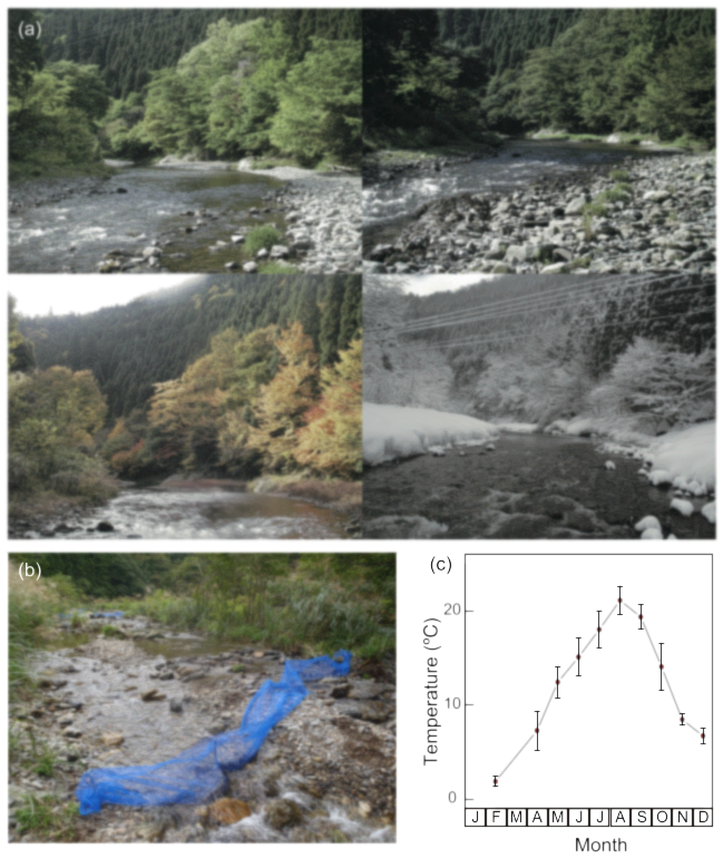
Fig. 1. (a) Typical views of the research site (upper left, May 2008; upper right, August 2007; lower left, November 2007; lower right, February 2011). (b) A view of the tributary from which fish were removed to estimate fish densities. (c) Seasonal changes in water temperature at the research site. The dots and error bars represent monthly averages and standard deviations, respectively, over the 5-year period from 2007 to 2011.
B. Research methods
a. Estimations of reductions in fish stomach contents
Reductions in the stomach contents of N. delicata were calculated as described previously (Nakagawa, 2017), as follows:
DR = 6 × exp(0.436 × T – 10.59) (Fn 1),
where the digestion ratio (DR) is the proportion of food digested after its ingestion after 6 h at T°C.
Reductions in the stomach contents of other fish species were estimated experimentally. Fish sampling was conducted from April 2014 to February 2015. Fish were collected using a cast net (7 mm mesh), a hand net (3 mm mesh), and electro-fishing equipment (delivering 300 V pulsed DC; LR-24 instrument; Smith-Root, Inc., Vancouver, WA, USA). All captured fish were transferred to the laboratory and acclimated for ≤ 3 days prior to experimentation in plastic tanks (W × D × H; 60 × 40 × 30 cm) filled with 48 L water at room temperature (~20ºC).
Experiments
The digestion ratios (DRs) of the foods ingested at 10, 15, 20, and 25ºC were calculated for all species. However, L. reinii and R. flumineus were inactive at 10ºC, and C. pollux was enfeebled at 25ºC. Therefore, DRs were not measured for these species at these temperatures. All fish were starved for 24 h to allow stomach evacuation prior to feeding for DR determination. At 12 h before feeding, each individual fish was placed in a plastic cage hanging on the wall of a plastic tank (W × D × H, 60 × 40 × 30 cm) filled with 48 L water at room temperature (~20ºC). The water temperature of the tank was gradually adjusted by < 5 ºC/h to attain the desired temperature using the combination of aquarium heater (POWER SAFE PRO 300W, Nisso, Osaka) and cooler with an internal thermostat (ZR-75E, Zensui, Osaka) for each experiment. The cage sizes (W × D × H) were 9 × 9 × 9 cm for small fish (≤ 8 cm in total length) and 15 × 15 × 10 cm for large fish (> 8 cm in total length). After the water reached the desired temperature, each fish was fed 10–40 thawed chironomid larvae (Chironomus sp.). The wet weight (ww, g) of the food was measured to the nearest 0.001 g and converted to dry weight (dw, g) using the following linear function: dw = 0.080ww; N = 12, r2 = 0.999, p < 0.001 (H. Nakagawa, unpublished). The dw of a single chironomid larva was 0.40±0.04 mg (mean ± SD). Food remaining on the bottom of the plastic case 10 min after the food was offered was salvaged, and its ww was deducted from the ww of the food initially provided. Each fish was removed from its rearing cage 6 or 12 h after feeding and immediately placed on a freezer to stop digestion. Data were collected from three or four individuals at each temperature and time. The ww of the individual fish was measured to the nearest 0.001 g. Then, each individual fish was dissected, and the food remaining in the stomach was weighed to the nearest 0.001 g after drying at 60°C for 24 h. For cyprinids and R. flumineus (Gobiidae), the stomach was defined as the portion of the intestine from the entrance of the digestive tract to the first bend because of the absence of a true stomach secreting hydrochloric acid and pepsin (Hofer, 1991). The stomachs of the other fish were defined as the true stomachs of the gastrointestinal tracts. The ww value for each individual fish was converted to a dw value using the following linear function: dw = 0.220 ww; N = 51, r2 = 0.984, p < 0.001 (H. Nakagawa, unpublished).
Statistical estimation
The temperature-dependent DR patterns were described using a generalized linear model (GLM) featuring a binomial error distribution and a logistic link function, extending the original method commonly used to estimate thermal effects on DR (Elliot, 1972). The original method estimates the relationship between the relative weight of the final compared with the initial stomach contents and the time after feeding at each temperature, as follows:
Fend / Fstart = exp(a1 – DR*t) (Fn 2),
where a1 is a constant, Fstart and Fend are the weights of food in the stomach at the start and end of a given time window, respectively, t is the time after feeding, and the slope DR* is the DR per unit time (i.e., the constant rate of digestion), which was termed the gastric evacuation rate in the study originally describing this method (Elliot, 1972). Thus, Fn 2 shows that the relationship between the DR* and temperature (T) can be evaluated by linear regression as follows:
DR* = a2 + bT (Fn 3),
where a2 and b are constants. The linear predictor for the GLM was derived by substituting Fn 3 into Fn 2 as follows:
Fend / Fstart = exp(a1 – a2t – bTt) (Fn 4).
In this function, the constant a2 represents the time-dependent decrease in stomach food content at 0ºC, and the constant b represents the temperature-dependent adjustment. In line with this analysis, the linear predictor was adapted to a logistic link function representing the ratio of the decrease in stomach contents, as follows:
Fend / Fstart = 1 / (1 + exp[–(a1 – a2t – bTt + offset term)]) (Fn 5).
The response variables were magnified by 1,000 in fitting to the GLM, because the binomial distribution assumes that the denominator of the response variable (Fend / Fstart) is an integral value. In our analysis, the time after feeding was treated as a categorical variable, because the time points used in these analyses (6 and 12 h) were too few in number to be considered continuous. The log (weight) of each fish served as an offset term reflecting adjustment of the fish body mass calculated prior to regression analyses using our original method. The r2 and adjusted r2 values generalized for GLM were calculated using the methods of Nagelkerke (1991) and Faraway (2006). The DR was thus defined as 1 − Fend / Fstart for a 1 g fish at each temperature evaluated over a defined experimental period (Table 1).
Table 1. The GLM results using the formula DR = 1 − (1/(1 + exp (− (a1 − a2t − bTt)))), where a1, a2 and b are constants, t is the time after feeding, T is the water temperature, and Tt is the T × t. The time after feeding was treated as a categorical variable (t = 6 or t = 12), because the time points used in these analyses were too few in number to be considered continuous. The DR was defined as 1 − Fend / Fstart for a 1 g fish at each temperature evaluated over a defined experimental period. Fstart and Fend are the weights of food in the stomach at the start and end of the experimental period, respectively. The r2 and adjusted r2 values generalized for GLM were calculated following the methods of Nagelkerke (1991) and Faraway (2006).
| Species | Zacco temminckii | Tribolodon hakonensis | Phoxinus oxycephalus | Liobagrus reinii | Rhinogobius flumineus | Cottus pollux | ||
|---|---|---|---|---|---|---|---|---|
| Estimate ± SE (P-value) | Intercept | 4.012 ± 1.106 (< 0.001) | 4.831 ± 1.203 (< 0.001) | 4.333 ± 0.937 (< 0.001) | 4.844 ± 1.348 (< 0.001) | 6.107 ± 1.998 (0.002) | -1.003 ± 1.259 (0.426) | |
| t | t = 12 | 1.088 ± 2.217 (0.624) | 5.453 ± 1.816 (0.003) | -0.817 ± 2.140 (0.703) | -0.250 ± 2.087 (0.905) | -3.772 ± 3.506 (0.282) | -4.351 ± 1.864 (0.020) | |
| Tt | t = 6 | 0.269 ± 0.068 (< 0.001) | 0.332 ± 0.064 (< 0.001) | 0.248 ± 0.055 (< 0.001) | 0.216 ± 0.066 (0.001) | 0.210 ± 0.091 (0.020) | -0.042 ± 0.087 (0.630) | |
| t = 12 | 0.374 ± 0.157 (0.017) | 0.118 ± 0.083 (0.155) | 0.539 ± 0.179 (0.003) | 0.310 ± 0.091 (0.001) | 0.510 ± 0.159 (0.001) | 0.284 ± 0.095 (0.003) | ||
| Null DF | 25 | 23 | 26 | 22 | 19 | 19 | ||
| Null deviance | 68.3 | 89.9 | 151.0 | 56.3 | 51.7 | 41.9 | ||
| Residual DF | 22 | 20 | 23 | 19 | 16 | 16 | ||
| Residual deviance | 18.3 | 40.7 | 61.3 | 19.1 | 18.4 | 30.2 | ||
| R2 | 0.925 | 0.900 | 0.971 | 0.884 | 0.885 | 0.516 | ||
| adjusted R2 | 0.914 | 0.884 | 0.967 | 0.865 | 0.862 | 0.419 | ||
b. Fish sampling
We performed fish sampling once each in August, October, and December 2008 and April and June 2009 to examine stomach contents. Sampling was performed at four different times each day (02:00–03:00, 08:00–09:00, 14:00–15:00, and 20:00–21:00), because we found that the stomach contents varied significantly over a 24 h period in our previous study (Nakagawa et al. 2012), and because several daily samplings were necessary to determine daily consumption rates (Elliot 1972). Three to seven individuals per sampling of each species were captured, but one sample of P. oxycephalus at 02:00 in October was available due to lost of samples. We used a cast net with a mesh size of 7 mm and a hand net with a mesh size of 3 mm for sampling. The captured fish were immediately anesthesia administered in a plastic tank with ice water, labeled, fixed in 10% formalin within two hours after catching, and transferred to the laboratory for analysis.
c. Estimation of daily consumption rates of fishes
The standard length (SL, mm) and ww of each fish were measured prior to stomach content analysis. The ww values were converted to dw values using a previously derived equation (dw = 0.235ww, N = 46, r2 = 0.996, p < 0.0001; Nakagawa, unpublished). The fish were then dissected and their stomach contents identified. Aquatic animals (fish and macroinvertebrates) removed from stomachs were generally identified to the species level; however, some were identified to the genus, subfamily, or family level, because complete taxonomic descriptions were not available. Algae, terrestrial plant seeds/fruits, terrestrial invertebrates, and fallen adults of aquatic insects were not identified to further taxonomic groups. Each prey item was dried on a hotplate (60°C) for more than 24 h and then weighed (dw, g). Rarefaction curves of the number of consumed prey items of various invertebrate taxa plotted against the number of dissected fish individuals were drawn using 1,000 resampling simulations to examine the effect of sample size on the observation rates of prey taxa. The richness of prey taxa were determined using the Chao estimator (Cardoso et al. 2015) for each fish species (Fig. 2).
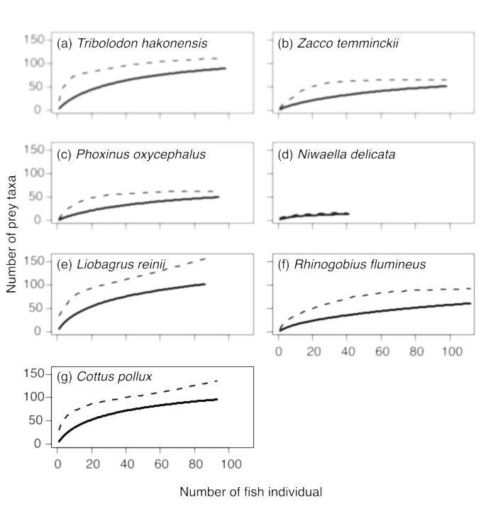
Fig. 2. Rarefaction curves of the number of consumed prey of various invertebrate taxa plotted against the number of dissected fish individuals. The number of prey was derived by stomach content analysis of each fish species. The solid and dashed lines indicate the observed and the richness of prey taxa determined using the Chao estimator (Cardoso et al. 2015), respectively.
The dw of each prey item consumed by the dominant fish was determined for each of the four 6 h sampling intervals following Elliot (1972) and Elliot and Person (1978):
Ct = (St − S0 e−RT)RT / (1 − e−RT) (Fn 6),
where Ct is the dw (g) of prey consumed per gram of fish dw over a sampling interval of t (h); S0 and St are the mean dw of prey in the stomach per gram of fish dw at the beginning and end, respectively, of the 6-h sampling interval; e is the base of the natural logarithm; and RT is the DR over the 6 h interval at T (°C).
d. Estimation of fish abundance, biomass, and microhabitat preference
The estimation of fish abundance (individuals/m2) were conducted at about 100 m upstream of the main sampling site of fishes and their prey at the main stream of the Yura river during each month that fish were sampled for stomach content analysis. The abundances in the main stream were calculated as the number of fish observed in the main stream using the line transect method × the finding rate. The finding rate of each fish was measured in a tributary near the main sampling site (≤ 5 m wet width) in September and December 2011 and April 2012. The finding rate was calculated as the observed number of fish individuals in the tributary divided by the density of each fish species. The observed number of fish individuals in the tributary was obtained by the line-transect method with the procedure that was the same as that conducted at the main stream. We estimated the density of fish species in the tributary each sampling month using the removal method (Zippin 1956) with an electro-fisher (LR-24; Smith-Root, Inc.). Fish sampling was repeated three to six times until the fish numbers were clearly decreased in each section. The total ww of each fish species was measured to the nearest gram to calculate the dw value as follows: dw = 0.220ww, N = 51, r2 = 0.984, p < 0.0001 (H. Nakagawa, unpublished). The mean dw of an individual fish was calculated by dividing the total mass of the fish by the density estimation for each fish species. The biomass (dw, g/m2) of each fish in the main stream was calculated as the fish abundance in the main stream × the mean dw of those individual fish. As the finding rate and line transect abundance estimates in the main stream were not concurrent, we used the finding rate from April to calculate densities in the main stream in April, the finding rate in September to calculate the main stream densities in June, August, and October, and the finding rate in December to calculate the main stream densities in December. Hibernation has been reported in N. delicata, in that these fish move into groundwater between autumn and spring (Kawanabe & Mizuno 1989) and do not occupy habitats in the main stream of the river. L. reinii has also been suggested to migrate into tributaries or cracks in the bedrock (H. Nakagawa, personal observations). Therefore, the densities, body masses, and daily consumption rates of N. delicata from autumn to spring (April, October, and December), and those of L. reinii in winter (December), were treated as zero. We surveyed the microhabitat uses of the fish (water depth, current speed, and substrate characteristics) at our research site at the times at which we made the line-transect observations, using the methods of Nakagawa (2014).
e. Sampling of invertebrates and descriptions of their microhabitats
Benthic invertebrates were collected using a Surber sampler (250 μm mesh) from 50 × 50 cm quadrats at an about 100 m reach in the main sampling site once every 2 months, at the same times that fish were collected for stomach content analysis. Six samples were collected from a pool, six from a riffle, and one from a riverbank bedrock habitat, reflecting the frequency of each habitat within the research site. Before sampling, microhabitat data (water depth, current speed, and substrate characteristics) were measured using the same methods as employed for fish observations (Nakagawa 2014). The samples were preserved in 99.5% ethanol and transferred to the laboratory. Benthic invertebrates were separated by passing the samples through 4 mm mesh and 1 mm mesh sieves. Then, all materials retained by the 4 mm mesh and one-eighth of the well-stirred material retained by the 1 mm mesh sieve were sorted and identified using a binocular microscope. The identification procedure used for benthic invertebrates was the same as that used for fish stomach content analysis. We drew rarefaction curves of the number of invertebrate taxa observed against the number of samples in the Surber nets at pool and riffle habitats, and the richness of prey taxa were calculated using the method described above for fish stomach content analysis, for each sampling month (Fig. 3).
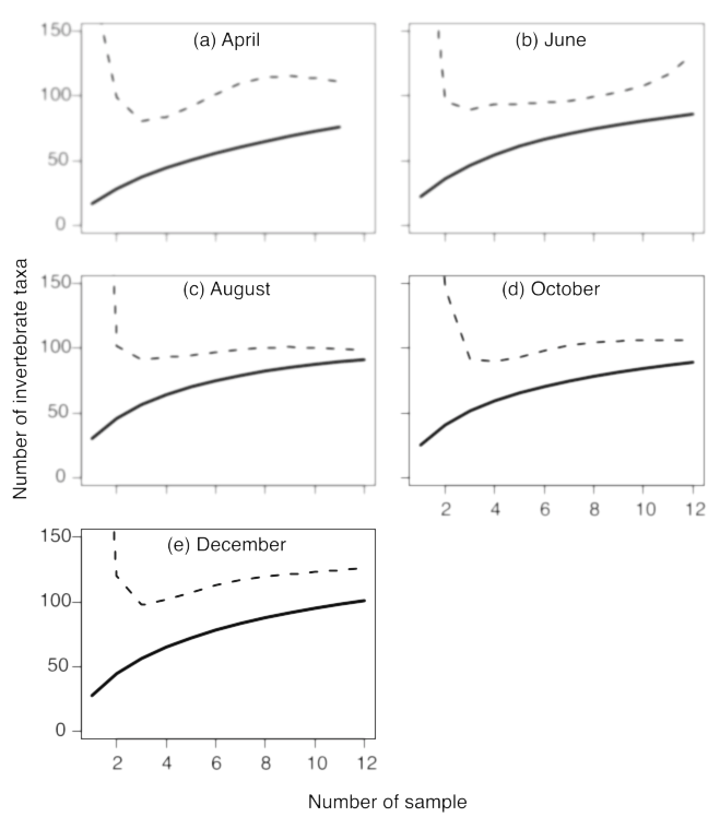
Fig. 3. Rarefaction curves of the number of invertebrate taxa against the number of quadrats sampled during at pool and riffle habitats each sampling month. Solid and dashed lines indicate the observed richness of prey taxa and the one calculated using the Chao estimator (Cardoso et al. 2015), respectively.
f. Estimation of invertebrate abundance, biomass, body mass, and production
Each identified invertebrate was dried on a hot plate (60°C) for more than 24 h and then weighed (dw, g). The total mass of each species/taxon was divided by the total quadrat area (0.25 m2 × 13) to calculate the biomass (g/m2) of each benthic invertebrate. The biomass and abundance of invertebrates retained by the 1 mm mesh sieve were adjusted by multiplying the numbers eightfold. The mean body mass (dw, g) of the benthic invertebrates was calculated by dividing the total mass of each species/taxon by the total number of individuals.
The daily production levels (the daily masses) of benthic invertebrates were determined by comparing the body mass at the start with that at the end of the four sampling periods (April–June, June–August, August–October, and October–December), as follows;
Pt = (Bt − B0) / B0 / t (Fn 7),
where Pt is the daily production per gram of invertebrate body mass (g/g prey/day) over a sampling interval t (days), and B0 and Bt are the mean body masses of a benthic invertebrate taxon at the start and end, respectively, of the sampling period. The daily production from December to April was not estimated, because the invertebrates species turnover at the study site during this period was very high (H. Nakagawa unpublished). If growth within any period was negative (perhaps because of emergence of an aquatic insect), the production of that invertebrate taxon was treated as zero. Although daily production of organisms is usually calculated as a unit area value (e.g., g/m2/day) rather than a unit mass value (e.g., Benke & Huryn 2006), we used the per mass value, because most theoretical studies on food webs have described predator consumption and prey production using per individual or per mass values (e.g., Yodzis & Innes 1992; McCann et al. 1998; Post et al. 2000; Kondoh 2003).
g. Sampling of algae
Samples of algae were collected from 12 randomly selected cobbles (minor axis > 10 cm) of riffle and pool habitats in the same areas where invertebrates were sampled and at the same times when fish stomach contents were analyzed. A latex plate with a 5 × 5 cm square opening was placed on a cobble, and algae were brushed out of the opening. The samples were placed on ice and frozen within 1 h. The samples were then transferred to the laboratory, dried on a hotplate (60°C) for over 24 h, oxidized at 600°C for 2 h in an oven, and analyzed for ash-free dw (g). The total ash-free dw of algae during each season was divided by the total quadrat area (0.0025 m2 × 12) to calculate the algal biomass (g/m2).
h. Estimation of dC and the C/P ratio
The dC of each fish species for each prey (dw, g/g predator/day) was calculated as the product of the daily consumption rate of the fish and the relative mass of the prey species in the fish stomach during each sampling month. The C/P ratio was calculated for each trophic link within each sampling period as follows:
C/Pt = ((dC0 + dCt) / 2) / Pt (Fn 8),
where C/Pt is the mean daily C/P ratio in a sampling interval t (days), Pt is the per gram daily production of prey, and dC0 and dCt are the dC values at the start and end of a seasonal sampling period, respectively. The dC and C/P values for each trophic link over the entire year were calculated as the mean values for all five sampling months and for the four sampling periods, respectively.
C. Data verification procedures
The data were manually digitized and checked for typographical errors by the investigators.
8. DATA STATUS
A. Latest update
16 July 2017
B. Metadata status
The metadata are complete for this period and stored with the data.
9. ACCESSIBILITY
A. License and usage rights
You are free to copy and redistribute the material in any medium or format, remix, transform, and build upon the material for any purpose, even commercially. You must give appropriate credit, provide a link to the license, and indicate if changes were made. You may do so in any reasonable manner, but not in any way that suggests the licensor endorses you or your use.
B. Contact
Hikaru Nakagawa
Field Science Education and Research Center, Kyoto University,1 Onojya, Miyama, Nantan, Kyoto, 601-0703, Japan, hikarunakagwa@icloud.com
C. Storage location
Raw data sheets and digital data are stored with H. Nakagawa on multiple hard drives in two physical locations.
10. DATA STATUS
A. Data tables
| Data file names | Description |
|---|---|
| Table_S1_taxa.csv | List of component taxa. |
| Table_S2_abundance.csv | Abundance (individuals/m2) of each component taxa in each season. |
| Table_S3_biomass.csv | Biomass (g-drymass/m2) of each component taxa in each season. |
| Table_S4_bodymass.csv | Bodymass (g-drymass) of each component taxa in each season. |
| Table_S5_microhabitat.csv | Environmental characters (Mean ± SD) of habitat of each component species in each season. |
| Table_S6_production.csv | Per mass daily production (g-drymass/g-bodymass/day) of each prey taxa in each season. |
| Table_S7_dC.csv | Per mass daily consumption rate (g-drymass/g-fishmass/day) of each fish species on each prey taxa in each season. |
| Table_S8_CP.csv | Ratio between the per mass predator consumption rates of each fish species and production rate of each prey taxa in each season. |
B. Format type
The data files are in UTF-8 text, comma delimited (csv).
C. Header information
Headers corresponding to variable names (see section 10.D) are included as the first row in the data file.
D. Variable definitions
| Variable name | Variable definition | Unit | Storage type | Precision | Reference |
|---|---|---|---|---|---|
| Fish species/prey taxa | Species of fishes or taxa of prey organisms | NA | Characters | NA | Table S1–8 |
| Order | Order of fishes or prey organisms | NA | Characters | NA | Table S1 |
| Family | Family of fishes or prey organisms | NA | Characters | NA | Table S1 |
| Genus | Genus of fishes or prey organisms | NA | Characters | NA | Table S1 |
| Species | Species of fishes or prey organisms | NA | Characters | NA | Table S1 |
| April_abundance | Abundance of fish species or prey organisms in April | individuals/m2 | Calculated value | 0.001 | Table S2 |
| June_abundance | Abundance of fish species or prey organisms in June | individuals/m2 | Calculated value | 0.001 | Table S2 |
| August_abundance | Abundance of fish species or prey organisms in August | individuals/m2 | Calculated value | 0.001 | Table S2 |
| October_abundance | Abundance of fish species or prey organisms in October | individuals/m2 | Calculated value | 0.001 | Table S2 |
| December_abundance | Abundance of fish species or prey organisms in December | individuals/m2 | Calculated value | 0.001 | Table S2 |
| April_biomass | Biomass of fish species or prey organisms in April | g/m2 | Calculated value | 0.000001 | Table S3 |
| June_biomass | Biomass of fish species or prey organisms in June | g/m2 | Calculated value | 0.000001 | Table S3 |
| August_biomass | Biomass of fish species or prey organisms in August | g/m2 | Calculated value | 0.000001 | Table S3 |
| October_biomass | Biomass of fish species or prey organisms in October | g/m2 | Calculated value | 0.000001 | Table S3 |
| December_biomass | Biomass of fish species or prey organisms in December | g/m2 | Calculated value | 0.000001 | Table S3 |
| April_bodymass | Bodymass of fish species or prey organisms in April | g | Calculated value | 0.000001 | Table S4 |
| June_bodymass | Bodymass of fish species or prey organisms in June | g | Calculated value | 0.000001 | Table S4 |
| August_bodymass | Bodymass of fish species or prey organisms in August | g | Calculated value | 0.000001 | Table S4 |
| October_bodymass | Bodymass of fish species or prey organisms in October | g | Calculated value | 0.000001 | Table S4 |
| December_bodymass | Bodymass of fish species or prey organisms in December | g | Calculated value | 0.000001 | Table S4 |
| Water depth in April | Water depth of microhabitat used by fish species or prey animals in April | cm/s | Calculated value | 0.01 | Table S5 |
| Water depth in June | Water depth of microhabitat used by fish species or prey animals in June | cm/s | Calculated value | 0.01 | Table S5 |
| Water depth in August | Water depth of microhabitat used by fish species or prey animals in August | cm/s | Calculated value | 0.01 | Table S5 |
| Water depth in October | Water depth of microhabitat used by fish species or prey animals in October | cm/s | Calculated value | 0.01 | Table S5 |
| Water depth in December | Water depth of microhabitat used by fish species or prey animals in December | cm/s | Calculated value | 0.01 | Table S5 |
| Upper column current velocity in April | Upper column current velocity of microhabitat used by fish species or prey animals in April | cm/s | Calculated value | 0.01 | Table S5 |
| Upper column current velocity in June | Upper column current velocity of microhabitat used by fish species or prey animals in June | cm/s | Calculated value | 0.01 | Table S5 |
| Upper column current velocity in August | Upper column current velocity of microhabitat used by fish species or prey animals in August | cm/s | Calculated value | 0.01 | Table S5 |
| Upper column current velocity in October | Upper column current velocity of microhabitat used by fish species or prey animals in October | cm/s | Calculated value | 0.01 | Table S5 |
| Upper column current velocity in December | Upper column current velocity of microhabitat used by fish species or prey animals in December | cm/s | Calculated value | 0.01 | Table S5 |
| Middle column current velocity in April | Middle column current velocity of microhabitat used by fish species or prey animals in April | cm/s | Calculated value | 0.01 | Table S5 |
| Middle column current velocity in June | Middle column current velocity of microhabitat used by fish species or prey animals in June | cm/s | Calculated value | 0.01 | Table S5 |
| Middle column current velocity in August | Middle column current velocity of microhabitat used by fish species or prey animals in August | cm/s | Calculated value | 0.01 | Table S5 |
| Middle column current velocity in October | Middle column current velocity of microhabitat used by fish species or prey animals in October | cm/s | Calculated value | 0.01 | Table S5 |
| Middle column current velocity in December | Middle column current velocity of microhabitat used by fish species or prey animals in December | cm/s | Calculated value | 0.01 | Table S5 |
| Bottom column current velocity in April | Bottom column current velocity of microhabitat used by fish species or prey animals in April | cm/s | Calculated value | 0.01 | Table S5 |
| Bottom column current velocity in June | Bottom column current velocity of microhabitat used by fish species or prey animals in June | cm/s | Calculated value | 0.01 | Table S5 |
| Bottom column current velocity in August | Bottom column current velocity of microhabitat used by fish species or prey animals in August | cm/s | Calculated value | 0.01 | Table S5 |
| Bottom column current velocity in October | Bottom column current velocity of microhabitat used by fish species or prey animals in October | cm/s | Calculated value | 0.01 | Table S5 |
| Bottom column current velocity in December | Bottom column current velocity of microhabitat used by fish species or prey animals in December | cm/s | Calculated value | 0.01 | Table S5 |
| Sand in April | Sand of microhabitat used by fish species or prey animals in April | dimensionless | Relative frequency | 0.01 | Table S5 |
| Sand in June | Sand of microhabitat used by fish species or prey animals in June | dimensionless | Relative frequency | 0.01 | Table S5 |
| Sand in August | Sand of microhabitat used by fish species or prey animals in August | dimensionless | Relative frequency | 0.01 | Table S5 |
| Sand in October | Sand of microhabitat used by fish species or prey animals in October | dimensionless | Relative frequency | 0.01 | Table S5 |
| Sand in December | Sand of microhabitat used by fish species or prey animals in December | dimensionless | Relative frequency | 0.01 | Table S5 |
| Gravel in April | Gravel of microhabitat used by fish species or prey animals in April | dimensionless | Relative frequency | 0.01 | Table S5 |
| Gravel in June | Gravel of microhabitat used by fish species or prey animals in June | dimensionless | Relative frequency | 0.01 | Table S5 |
| Gravel in August | Gravel of microhabitat used by fish species or prey animals in August | dimensionless | Relative frequency | 0.01 | Table S5 |
| Gravel in October | Gravel of microhabitat used by fish species or prey animals in October | dimensionless | Relative frequency | 0.01 | Table S5 |
| Gravel in December | Gravel of microhabitat used by fish species or prey animals in December | dimensionless | Relative frequency | 0.01 | Table S5 |
| Cobble in April | Cobble of microhabitat used by fish species or prey animals in April | dimensionless | Relative frequency | 0.01 | Table S5 |
| Cobble in June | Cobble of microhabitat used by fish species or prey animals in June | dimensionless | Relative frequency | 0.01 | Table S5 |
| Cobble in August | Cobble of microhabitat used by fish species or prey animals in August | dimensionless | Relative frequency | 0.01 | Table S5 |
| Cobble in October | Cobble of microhabitat used by fish species or prey animals in October | dimensionless | Relative frequency | 0.01 | Table S5 |
| Cobble in December | Cobble of microhabitat used by fish species or prey animals in December | dimensionless | Relative frequency | 0.01 | Table S5 |
| Boulder in April | Boulder of microhabitat used by fish species or prey animals in April | dimensionless | Relative frequency | 0.01 | Table S5 |
| Boulder in June | Boulder of microhabitat used by fish species or prey animals in June | dimensionless | Relative frequency | 0.01 | Table S5 |
| Boulder in August | Boulder of microhabitat used by fish species or prey animals in August | dimensionless | Relative frequency | 0.01 | Table S5 |
| Boulder in October | Boulder of microhabitat used by fish species or prey animals in October | dimensionless | Relative frequency | 0.01 | Table S5 |
| Boulder in December | Boulder of microhabitat used by fish species or prey animals in December | dimensionless | Relative frequency | 0.01 | Table S5 |
| Bedrock in April | Bedrock of microhabitat used by fish species or prey animals in April | dimensionless | Relative frequency | 0.01 | Table S5 |
| Bedrock in June | Bedrock of microhabitat used by fish species or prey animals in June | dimensionless | Relative frequency | 0.01 | Table S5 |
| Bedrock in August | Bedrock of microhabitat used by fish species or prey animals in August | dimensionless | Relative frequency | 0.01 | Table S5 |
| Bedrock in October | Bedrock of microhabitat used by fish species or prey animals in October | dimensionless | Relative frequency | 0.01 | Table S5 |
| Bedrock in December | Bedrock of microhabitat used by fish species or prey animals in December | dimensionless | Relative frequency | 0.01 | Table S5 |
| April_June_production | Daily production of prey animals from April to June | g/g-bodymass/day | Calculated value | 0.000001 | Table S6 |
| June_August_production | Daily production of prey animals from June to August | g/g-bodymass/day | Calculated value | 0.000001 | Table S6 |
| August_October_production | Daily production of prey animals from August to October | g/g-bodymass/day | Calculated value | 0.000001 | Table S6 |
| October_December_production | Daily production of prey animals from October to December | g/g-bodymass/day | Calculated value | 0.000001 | Table S6 |
| Tribolodon hakonensis in April | Daily consumption rate of fish species on prey taxa in April | g/g-fishmass/day | Calculated value | 0.000001 | Table S7 |
| Phoxnus oxycephalus in April | Daily consumption rate of fish species on prey taxa in April | g/g-fishmass/day | Calculated value | 0.000001 | Table S7 |
| Zacco temminckii in April | Daily consumption rate of fish species on prey taxa in April | g/g-fishmass/day | Calculated value | 0.000001 | Table S7 |
| Niwaella delicata in April | Daily consumption rate of fish species on prey taxa in April | g/g-fishmass/day | Calculated value | 0.000001 | Table S7 |
| Liobagrus reinii in April | Daily consumption rate of fish species on prey taxa in April | g/g-fishmass/day | Calculated value | 0.000001 | Table S7 |
| Rhinogobius flumineus in April | Daily consumption rate of fish species on prey taxa in April | g/g-fishmass/day | Calculated value | 0.000001 | Table S7 |
| Cottus pollux in April | Daily consumption rate of fish species on prey taxa in April | g/g-fishmass/day | Calculated value | 0.000001 | Table S7 |
| Tribolodon hakonensis in June | Daily consumption rate of fish species on prey taxa in June | g/g-fishmass/day | Calculated value | 0.000001 | Table S7 |
| Phoxnus oxycephalus in June | Daily consumption rate of fish species on prey taxa in June | g/g-fishmass/day | Calculated value | 0.000001 | Table S7 |
| Zacco temminckii in June | Daily consumption rate of fish species on prey taxa in June | g/g-fishmass/day | Calculated value | 0.000001 | Table S7 |
| Niwaella delicata in June | Daily consumption rate of fish species on prey taxa in June | g/g-fishmass/day | Calculated value | 0.000001 | Table S7 |
| Liobagrus reinii in June | Daily consumption rate of fish species on prey taxa in June | g/g-fishmass/day | Calculated value | 0.000001 | Table S7 |
| Rhinogobius flumineus in June | Daily consumption rate of fish species on prey taxa in June | g/g-fishmass/day | Calculated value | 0.000001 | Table S7 |
| Cottus pollux in June | Daily consumption rate of fish species on prey taxa in June | g/g-fishmass/day | Calculated value | 0.000001 | Table S7 |
| Tribolodon hakonensis in August | Daily consumption rate of fish species on prey taxa in August | g/g-fishmass/day | Calculated value | 0.000001 | Table S7 |
| Phoxnus oxycephalus in August | Daily consumption rate of fish species on prey taxa in August | g/g-fishmass/day | Calculated value | 0.000001 | Table S7 |
| Zacco temminckii in August | Daily consumption rate of fish species on prey taxa in August | g/g-fishmass/day | Calculated value | 0.000001 | Table S7 |
| Niwaella delicata in August | Daily consumption rate of fish species on prey taxa in August | g/g-fishmass/day | Calculated value | 0.000001 | Table S7 |
| Liobagrus reinii in August | Daily consumption rate of fish species on prey taxa in August | g/g-fishmass/day | Calculated value | 0.000001 | Table S7 |
| Rhinogobius flumineus in August | Daily consumption rate of fish species on prey taxa in August | g/g-fishmass/day | Calculated value | 0.000001 | Table S7 |
| Cottus pollux in August | Daily consumption rate of fish species on prey taxa in August | g/g-fishmass/day | Calculated value | 0.000001 | Table S7 |
| Tribolodon hakonensis in October | Daily consumption rate of fish species on prey taxa in October | g/g-fishmass/day | Calculated value | 0.000001 | Table S7 |
| Phoxnus oxycephalus in October | Daily consumption rate of fish species on prey taxa in October | g/g-fishmass/day | Calculated value | 0.000001 | Table S7 |
| Zacco temminckii in October | Daily consumption rate of fish species on prey taxa in October | g/g-fishmass/day | Calculated value | 0.000001 | Table S7 |
| Niwaella delicata in October | Daily consumption rate of fish species on prey taxa in October | g/g-fishmass/day | Calculated value | 0.000001 | Table S7 |
| Liobagrus reinii in October | Daily consumption rate of fish species on prey taxa in October | g/g-fishmass/day | Calculated value | 0.000001 | Table S7 |
| Rhinogobius flumineus in October | Daily consumption rate of fish species on prey taxa in October | g/g-fishmass/day | Calculated value | 0.000001 | Table S7 |
| Cottus pollux in October | Daily consumption rate of fish species on prey taxa in October | g/g-fishmass/day | Calculated value | 0.000001 | Table S7 |
| Tribolodon hakonensis in December | Daily consumption rate of fish species on prey taxa in December | g/g-fishmass/day | Calculated value | 0.000001 | Table S7 |
| Phoxnus oxycephalus in December | Daily consumption rate of fish species on prey taxa in December | g/g-fishmass/day | Calculated value | 0.000001 | Table S7 |
| Zacco temminckii in December | Daily consumption rate of fish species on prey taxa in December | g/g-fishmass/day | Calculated value | 0.000001 | Table S7 |
| Niwaella delicata in December | Daily consumption rate of fish species on prey taxa in December | g/g-fishmass/day | Calculated value | 0.000001 | Table S7 |
| Liobagrus reinii in December | Daily consumption rate of fish species on prey taxa in December | g/g-fishmass/day | Calculated value | 0.000001 | Table S7 |
| Rhinogobius flumineus in December | Daily consumption rate of fish species on prey taxa in December | g/g-fishmass/day | Calculated value | 0.000001 | Table S7 |
| Cottus pollux in December | Daily consumption rate of fish species on prey taxa in December | g/g-fishmass/day | Calculated value | 0.000001 | Table S7 |
| Tribolodon hakonensis in April June | Ratio between per mass rates of daily consumption of fish species and daily production of prey animals from April to June | dimensionless | Calculated value | 0.000001 | Table S8 |
| Phoxnus oxycephalus in April June | Ratio between per mass rates of daily consumption of fish species and daily production of prey animals from April to June | dimensionless | Calculated value | 0.000001 | Table S8 |
| Zacco temminckii in April June | Ratio between per mass rates of daily consumption of fish species and daily production of prey animals from April to June | dimensionless | Calculated value | 0.000001 | Table S8 |
| Niwaella delicata in April June | Ratio between per mass rates of daily consumption of fish species and daily production of prey animals from April to June | dimensionless | Calculated value | 0.000001 | Table S8 |
| Liobagrus reinii in April June | Ratio between per mass rates of daily consumption of fish species and daily production of prey animals from April to June | dimensionless | Calculated value | 0.000001 | Table S8 |
| Rhinogobius flumineus in April June | Ratio between per mass rates of daily consumption of fish species and daily production of prey animals from April to June | dimensionless | Calculated value | 0.000001 | Table S8 |
| Cottus pollux in April June | Ratio between per mass rates of daily consumption of fish species and daily production of prey animals from April to June | dimensionless | Calculated value | 0.000001 | Table S8 |
| Tribolodon hakonensis in June August | Ratio between per mass rates of daily consumption of fish species and daily production of prey animals from June to August | dimensionless | Calculated value | 0.000001 | Table S8 |
| Phoxinus oxycephalus in June August | Ratio between per mass rates of daily consumption of fish species and daily production of prey animals from June to August | dimensionless | Calculated value | 0.000001 | Table S8 |
| Zacco temminckii in June August | Ratio between per mass rates of daily consumption of fish species and daily production of prey animals from June to August | dimensionless | Calculated value | 0.000001 | Table S8 |
| Niwaella delicata in June August | Ratio between per mass rates of daily consumption of fish species and daily production of prey animals from June to August | dimensionless | Calculated value | 0.000001 | Table S8 |
| Liobagrus reinii in June August | Ratio between per mass rates of daily consumption of fish species and daily production of prey animals from June to August | dimensionless | Calculated value | 0.000001 | Table S8 |
| Rhinogobius flumineus in June August | Ratio between per mass rates of daily consumption of fish species and daily production of prey animals from June to August | dimensionless | Calculated value | 0.000001 | Table S8 |
| Cottus pollux in June August | Ratio between per mass rates of daily consumption of fish species and daily production of prey animals from June to August | dimensionless | Calculated value | 0.000001 | Table S8 |
| Tribolodon hakonensis in August October | Ratio between per mass rates of daily consumption of fish species and daily production of prey animals from August to October | dimensionless | Calculated value | 0.000001 | Table S8 |
| Phoxnus oxycephalus in August October | Ratio between per mass rates of daily consumption of fish species and daily production of prey animals from August to October | dimensionless | Calculated value | 0.000001 | Table S8 |
| Zacco temminckii in August October | Ratio between per mass rates of daily consumption of fish species and daily production of prey animals from August to October | dimensionless | Calculated value | 0.000001 | Table S8 |
| Niwaella delicata in August October | Ratio between per mass rates of daily consumption of fish species and daily production of prey animals from August to October | dimensionless | Calculated value | 0.000001 | Table S8 |
| Liobagrus reinii in August October | Ratio between per mass rates of daily consumption of fish species and daily production of prey animals from August to October | dimensionless | Calculated value | 0.000001 | Table S8 |
| Rhinogobius flumineus in August October | Ratio between per mass rates of daily consumption of fish species and daily production of prey animals from August to October | dimensionless | Calculated value | 0.000001 | Table S8 |
| Cottus pollux in August October | Ratio between per mass rates of daily consumption of fish species and daily production of prey animals from August to October | dimensionless | Calculated value | 0.000001 | Table S8 |
| Tribolodon hakonensis in October December | Ratio between per mass rates of daily consumption of fish species and daily production of prey animals from October to December | dimensionless | Calculated value | 0.000001 | Table S8 |
| Phoxnus oxycephalus in October December | Ratio between per mass rates of daily consumption of fish species and daily production of prey animals from October to December | dimensionless | Calculated value | 0.000001 | Table S8 |
| Zacco temminckii in October December | Ratio between per mass rates of daily consumption of fish species and daily production of prey animals from October to December | dimensionless | Calculated value | 0.000001 | Table S8 |
| Niwaella delicata in October December | Ratio between per mass rates of daily consumption of fish species and daily production of prey animals from October to December | dimensionless | Calculated value | 0.000001 | Table S8 |
| Liobagrus reinii in October December | Ratio between per mass rates of daily consumption of fish species and daily production of prey animals from October to December | dimensionless | Calculated value | 0.000001 | Table S8 |
| Rhinogobius flumineus in October December | Ratio between per mass rates of daily consumption of fish species and daily production of prey animals from October to December | dimensionless | Calculated value | 0.000001 | Table S8 |
| Cottus pollux in October December | Ratio between per mass rates of daily consumption of fish species and daily production of prey animals from October to December | dimensionless | Calculated value | 0.000001 | Table S8 |
11. SUPPLEMENTALY INFORMATION
We calculated the dC and C/P values for 1,281 (7 × 183) pairs of fish and 546 (7 × 78) pairs of invertebrates, respectively, both annually and seasonally. Woodward et al. (2005) described a quantitative food web in a small stream using an approach similar to ours and discussed potential concerns associated with taxonomic resolution, seasonality, and sample size when analyzing a complex food web. Oversimplification and poor taxonomic resolution (especially of organisms at lower trophic levels of an empirical food web) have been repeatedly criticized in debates on the consistency between observation and theory (e.g., Winemiller & Layman 2005; Woodward et al. 2005). In the present study, algae, terrestrial plant seeds/fruits, terrestrial invertebrates, and fallen adult aquatic insects were not identified to the species level, but most invertebrates were identified to the species level with the exception of the Chilonomidae. The efficiency of detection of trophic links depends on the sample size, especially when interactions are weak (Woodward et al. 2005). A sufficiently large sample size is necessary when analyzing patterns in a complex food web. To cover the diversity of prey invertebrate species adequately, we sampled both fish and invertebrates in a manner reflecting the spatiotemporal variations that we had evaluated previously at the same research site; we thus used known fish–prey interaction patterns (Nakagawa et al. 2012). However, the rarefaction curves and species diversity estimates (Chao estimates) indicated that we failed to detect approximately 12.5–34.6% and 7.6–35.1% of the total number of prey species detected in the stomach contents of each fish species and the total number of invertebrates present during each season, respectively. Therefore, the mean dC and C/P values may have been overestimated in our study. Especially, the C/P ratios in June and August require careful interpretation, because the positive value of the interaction strength was estimated for only a small number of links.
In this study, the sample of invertebrates for density estimation were preserved in 99.5% ethanol. Several studies reported that invertebrates within high grade alcohol decrease about 10–20% of those dry mass in a few weeks or longer preservation, while not formaldehyde (e.g., Howmiller 1972; Leuven et al. 1985). Therefore, biomass of invertebrates and estimates using the biomass data (i.e., body mass and production of invertebrates) may be underestimated within a range about 10–20%, and the C/P ratios may be overestimated within a range about 10–20%due to the underestimate of the production in this study.
Consistency between the definitions of empirical values and theoretical parameters is important when interpreting food web data ( Laska & Wootton 1998; Berlow et al. 1999, 2004; Wootton & Emmerson 2005). The dC and C/P estimates used in this study generally match the definitions employed in theoretical models describing a food web as a material/energy flow network (e.g., Polovina 1985; Yodzis & Innes 1992; Pauly et al. 2000). In contrast, to match data to theoretical models that represent food webs by numerical changes in their components (i.e., abundance-based models) (e.g., Holling 1959; May 1981; Pimm 1979), additional calculations are needed such as data correction of the empirical values by body mass of predator and/or prey species. In addition, these two empirical values do not take into account indirect effects such as the trophic cascade from the top predator species down to the bottom prey species (Power 1990; Carpenter & Kitchell 1993) or intraguild competition between fish and invertebrates (Polis & Holt 1992; Holt & Polis 1997). Therefore, the values may not compare well with empirical estimates or theoretical parameters of interaction strengths, defined as net effects among interacting component species. Examples of empirical estimates include Paine’s index and the dynamic index employed in empirical studies ( Laska & Wootton 1998; Wootton & Emmerson 2005). An example of a theoretical parameter is the Jacobian matrix used in theoretical studies (May 1972, 1981).
12. ACKNOWLEDGEMENTS
We thank Kirk O. Winemiller for a kind response to our sudden request for comments to our manuscript. We thank Takuya Sato, Michio Kondoh, Hiroyuki Togashi, and Komei Kadowaki for their numerous useful comments. We thank Kazutaka Ohta, Akifumi S. Tanabe, Satoshi Yamamoto, Yoshikazu Kato, Masaki Yasugi, Yoichiro Sakai, Masaru Sakai, Seigo Kawase, Ryouichi Tabata, Shuhei Umeda, Yoshiko Yamane, Mitsunori Nakano, Daiki Okumura, Sei Kawabata, and Takehiro Inui for assistance with the field surveys. We thank the staff of the Ashiu Forest Research Station and the Fisheries Cooperative of Miyama, Kyoto, Japan. This study was supported by Global COE Program A06 ‘Formation of a Strategic Base for Biodiversity and Evolutionary Research: from Genome to Ecosystem’ and Grant in Aid for Scientific Research (Nos. 1960224, 21254003) from the Ministry of Education, Culture, Sports and Technology, Japan.
13. REFFERENCES
Bascompte, J., Melian, C. J. & Sala, E. (2005) Interaction strength combinations and the overfishing of a marine food web. Proceedings of the National Academy of Sciences, 102, 5443–5447
Benke, A. C. & Huryn, A. D. (2006) Secondary production of macroinvertebrates. Methods in Stream Ecology 2nd edn. (eds F. R. Hauer & G. A. Lamberti) pp. 691–710. Elsevier, London, UK
Berlow, E. R., Navarrete, S. A., Briggs, C. J., Power, M. E. & Menge, B. A. (1999) Quantifying variation in the strength of species interactions. Ecology, 80, 2206–2224
Berlow, E. R., Newtel, A., Cohen, J. E., de Ruiter, P. C., Ebenman, B., Emmerson, M., Kokkoris, G. D., Logofet, D. O., McKane, A. J., Montoya, J. M. & Petchey, O. (2004) Interaction strengths in food webs: issues and opportunities. Journal of Animal Ecology, 73, 585–598
Cardoso, P., Rigal, F. & Carvalho, J. C. (2015) BAT – Biodiversity Assessment Tools, an R package for the measurement and estimation of alpha and beta taxon, phylogenetic and functional diversity. Methods in Ecology and Evolution, 6, 232–236
Carpenter, S. J. & Kitchell, J. F. (1993) The trophic cascade in lakes. Cambridge University Press, Cambridge, UK
Elliot, J. M. (1972) Rates of gastric evacuation in brown trout, Salmo trutta L. Freshwater Biology, 2, 1–18
Elliot, J. M. & Person, L. (1978) The estimation of daily rates of food consumption for fish. Journal of Animal Ecology, 47, 977–991
Elton, C. (1927) Animal ecology. Sidgwick and Jackson, Ltd, London, UK
Faraway, J. J. (2006) Extending the linear model with R: Generalized litenar, mixed effects and nonparametric regression models. Chapman and Hall, London, UK
Gardner, M. R. & Ashby, W. R. (1970) Connectance of large, dynamical (cybernetic) systems: Critical values for stability. Nature, 228, 784
Hofer, R. (1991) Digestion. Cyprinid fishes: Systematics, biology and exploitation (eds I. J. Winfield, and J. S. Nelson) pp. 413–425. Chapman and Hall, London, UK
Holling, C. S. (1959) Some characteristics of simple types of predation and parasitism. Canadian Entomology, 91, 113–133
Holt, R. D. & Polis, G. A. (1997) Theoretical framework for intraguild predation. The American Naturalist, 149, 745–764
Howmiller, R. P. (1972) Effects of preservatives on weights of some common macorbenthic invertebrates. Transactions of the American Fisheries Society, 101, 743–746
Kawanabe, H. & Mizuno, N. (1989) Freshwater fishes of Japan. YAMA–KEI Pub Co Ltd, Tokyo, Japan. (in Japanese)
Kondoh, M. (2003) Foraging adaptation and the relationship between food-web complexity and stability. Science, 299, 1388–1391
Laska, M. S. & Wootton, J. T. (1998) Theoretical concepts and empirical approaches to measuring interaction strength. Ecology, 79, 461–476
Leuven, R. S. E. W., Brock, T. C. M. & van Druten, H. A. M. (1985) Effects of preservation on dry- and ash-free dry weight biomass of some common aquatic macro-invertebrates. Hydrobiologia, 127, 151–159
May, R. M. (1972) Will a large complex system be stable? Nature, 238, 413–414
May, R. M. (1981) Theoretical Ecology 2nd ed. Blackwell, Oxford, London
McCann, K., Hastings, A. & Huxel, G. R. (1998) Weak trophic interactions and the balance of nature. Nature, 395, 794–798
McCann, K. S. (2000) The diversity–stability debate. Nature, 405, 228–233
Nakagawa, H., Yamane, H., Yasugi, M., Fujita, T., Yokoi, K., Ashiwa, H., Kitada, N., Takano, H., Suzuki, N., Kishimoto, J., Maeda, H., Yamano, H., Ito, T., Maruyama, H., Tominaga, K., Hatakeyama, E., Goto, M. & Takahashi, D. (2012) Diel changes in resource use and diet overlap in temperate stream fishes. Ecological Research, 27, 417–426
Nakagawa, H. (2014) Contribution of environmental and spatial factors to the structure of stream fish assemblages at different spatial scales. Ecology of Freshwater Fish, 23, 208–223
Nakagawa, H. (2017) Temperature-dependent gastric evacuation rate of the Japanese delicate loach Niwaella delicata (Cobitidae), Ichthyologycal Research, in press
Nagelkerke, N. J. D. (1991) A note on a general definition of the coefficient of determination. Biometrika, 78, 691–692
Pauly, D., Christensen, V, Walters, C. (2000) Ecopath, Ecosim, and Ecospace as tools for evaluating ecosystem impact of fisheries. ICES Journal of Marine Science, 57, 697–706
Pimm, S. L. (1979) The structure of food webs. Theoretical Population Biology, 16, 144–158
Polis, G. A. & Holt, R. D. (1992) Intraguild predation: dynamics of complex trophic interactions. Trends in Ecology and Evolution, 7, 151–154
Polis, G. A. & Winemiller K. O. (1996) Food webs; Integration of Patterns & Dynamics. Chapman & Hall, New York, USA
Polovina, J. J. (1985) An approach to estimate an ecosystem box model. U. S. Fisheries Bulletin, 83, 457–460
Post, D. M., Conners, M. E. & Goldberg, D. S. (2000) Prey preference by a top predator and the stability of linked food chains. Ecology, 81, 8–14
Power, M. E. (1990) Effects of fish in river food webs. Science, 250, 811–814
Rossberg, A. G. (2013) Food Webs and Biodiversity: Foundations, Models, Data. John Wiley & Sons, West Sussex, UK
Winemiller, K. O. & Layman, C. A. (2005) Food web science: moving on the path from abstraction to prediction. Dynamic food webs: multispecies assemblages, ecosystem development and environmental change (eds P. C. de Ruiter, V. Wolters & J. C. Moore), pp. 10–23. Academic Press, Amsterdam, Netherlands
Woodward, G., Speirs, D. C. & Hildrew, A. G. (2005) Quantification and resolution of a complex, size-structured food web. In: Advances in Ecological Research 36 (ed H. Caswell), pp. 85–131, Academic Press, Amsterdam, Netherlands
Wootton, J. T. & Emmerson, M. (2005) Measurement of interaction strength in nature. Annual Review of Ecology, Evolution, and Systematics, 36, 419–444
Yodzis, P. & Innes, S. (1992) Body size and consumer-resource dynamics. American Naturalist, 139, 1151–1175
Zippin, C. (1956) The removal method of population estimation. Journal of Wildlife Management, 22, 82–90
